Introducing The Visual Data Modeler

The new Visual Data Modeler makes visualizing and modifying your table schema easier than ever. This new feature in Backendless Database is another powerful tool for simplifying the app development process.

An often-overlooked but extremely vital part of any app’s development is deciding how to structure your database. Haphazardly throwing a database together can lead to a complicated jumbled mess of a database once data starts being collected.

One of the first critical tasks when designing an app is architecting (designing) your database. For many developers, this means breaking out the whiteboard and occasionally ending up with something like…

The Visual Data Modeler is here to save your sanity.

This new feature was built to make it as easy as possible to visualize your data tables’ relationships with one another. That is, to see which columns connect each table to each other.

To demonstrate how this works, let’s walk through a quick example.

Visual Data Modeler In Action

We are going to work with a database containing three tables: Country, City, and CountryLanguage.

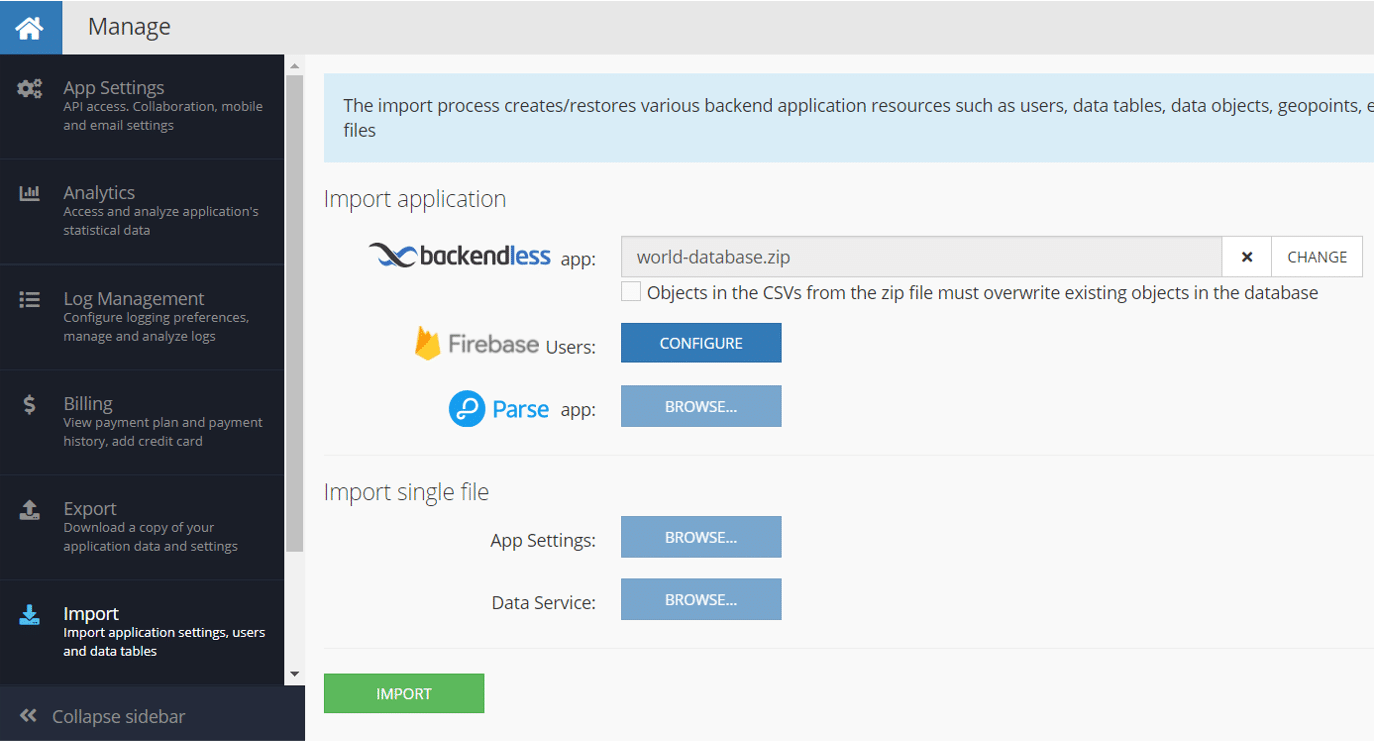
You can download the data we will be working with here. To follow along, import the data into any Backendless app:

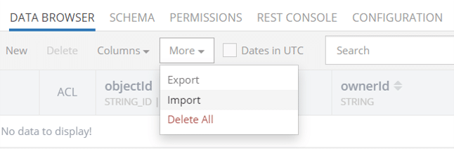
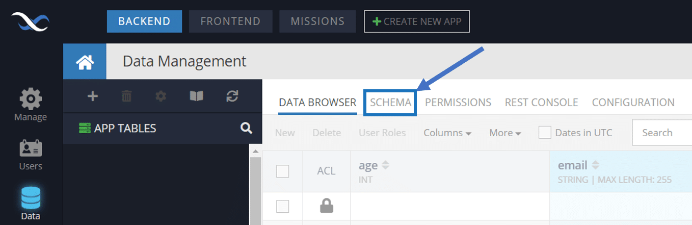
Once you’ve imported the data, you can access each table’s schema here:

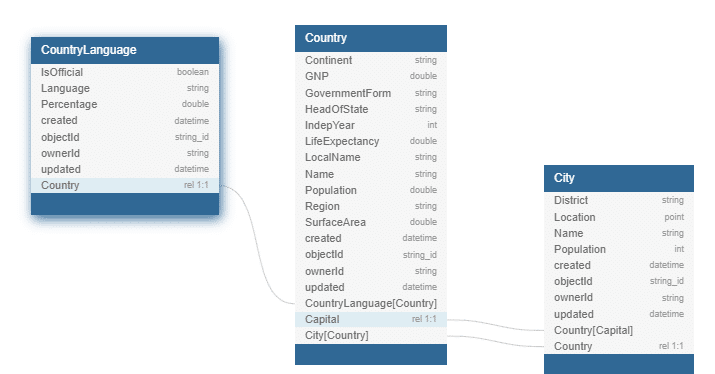
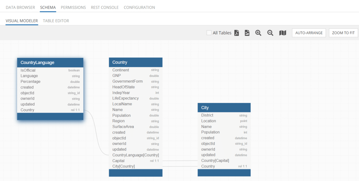
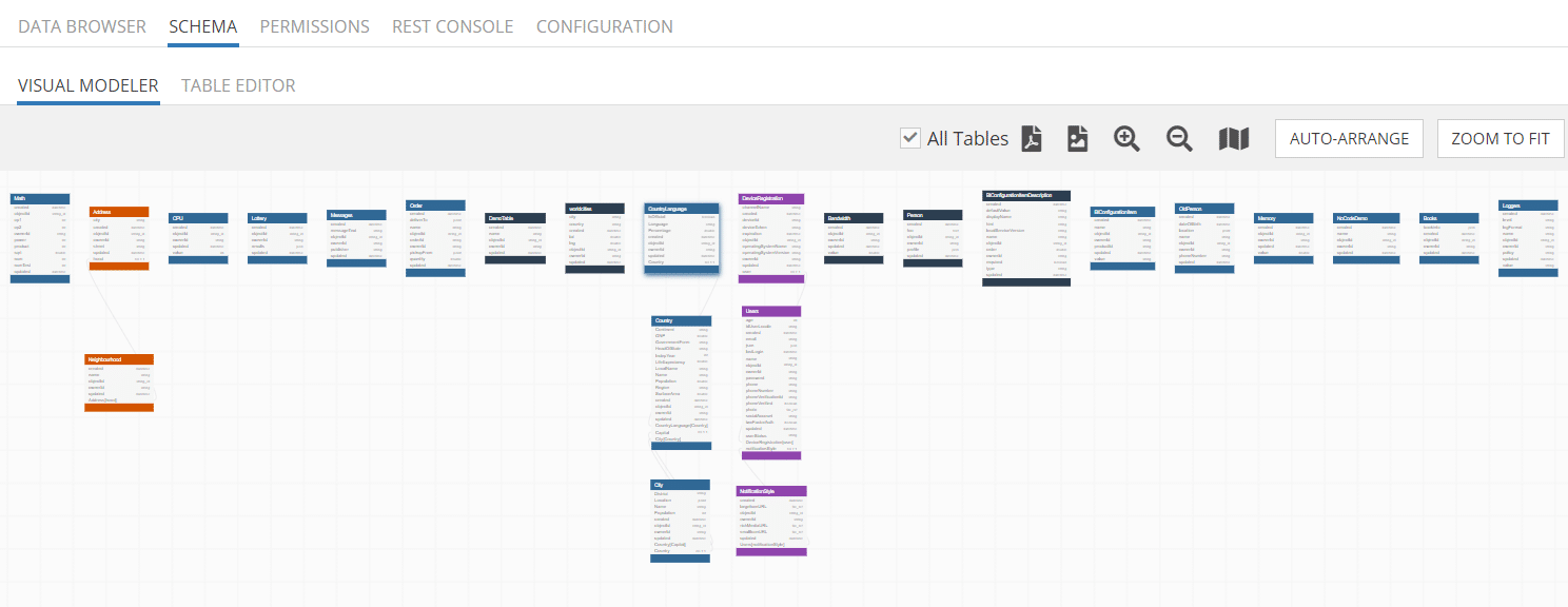
The first thing you will see is the visual schema model, automatically generated by Backendless based on the imported data:

The top-right menu bar gives you several useful options. The first is a checkbox for All Tables; when checked, all of the tables in your database will be visible.

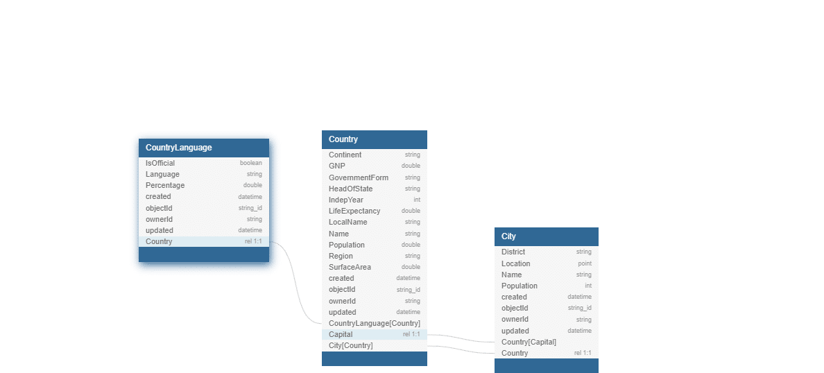
Next on the menu, after the All Tables checkbox, are the Export to PDF and Export to PNG buttons. An export of our CountryLanguage model looks like this:

The Auto-Arrange button will automatically lay out your tables in a way that makes it easier for you to see relationships between tables. If you had previously edited the arrangement of your tables in this view, Auto-Arrange will overwrite your changes.

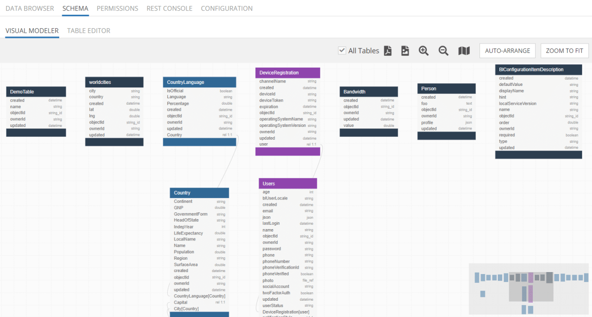
Zoom To Fit will bring all of your tables into one view. As you can see, color-coding your tables becomes quite useful as your number of data tables grows:

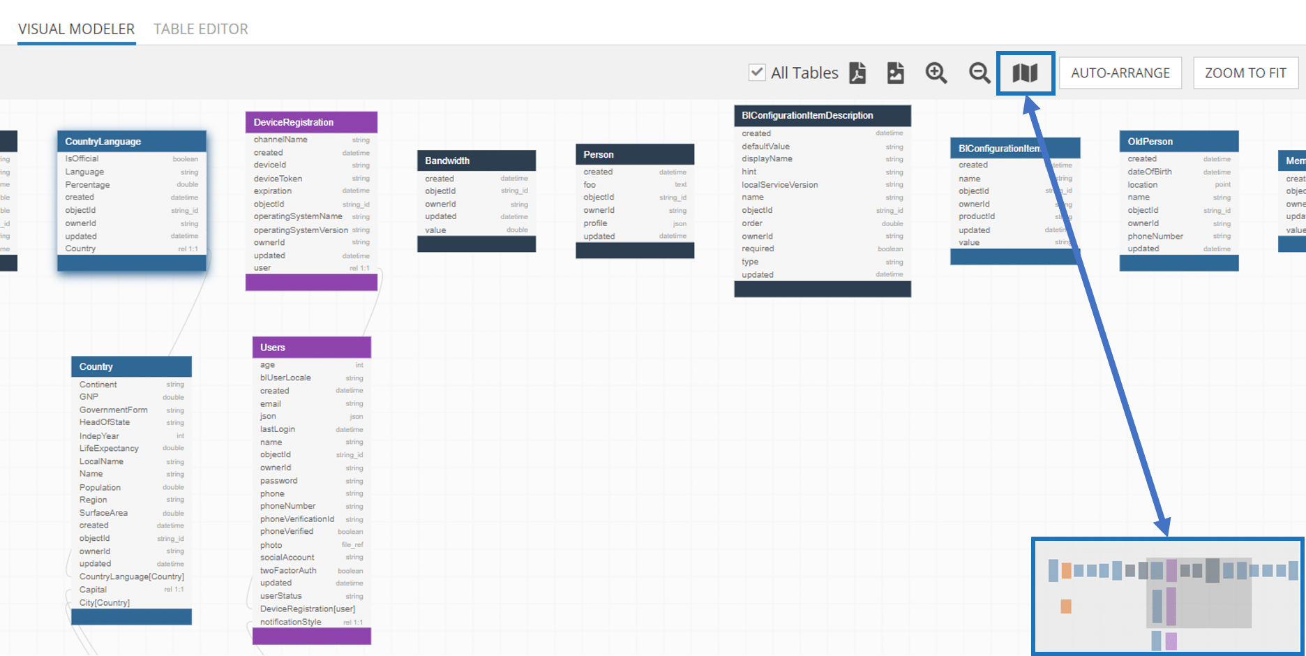
When you zoom in on the map or click the Map icon, you will pull up the map overlay in the bottom right corner. This will help you navigate around your tables as your database grows.

Modify Tables

Speaking of color-coding, let’s look at everything we can do with a table right in the Modeler.

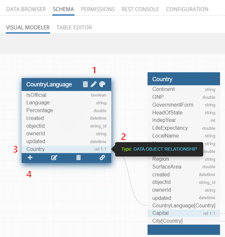
1. At the top of each table, you will see three options: delete, edit, and change color. The top delete button will delete the entire table. The top edit button allows you to rename the table (all existing relations will remain intact). You may choose from nine colors in the color changer.
2. When you hover over any column in a table, you will see the column type as well as any modifications (such as text length limits) and constraints (such as “Not Null”).
3. When you select a column in a table, the four options will appear on the bottom bar (see 4).
4. In order from left to right, we have:
   1. Add a new column
   2. Edit selected column
   3. Delete selected column
   4. Create relation (illustrated below)

Understanding Data Relations

Let’s do a quick-and-dirty explanation of how to understand data relations if you’ve never worked with database structure before. We’ll look back at the relations that have been created for our example tables and compare to their real-world connections.

Country

The Country table connects to the City table through two columns: Capital and Country. The Capital column is a 1:1 (one-to-one) relation, stored in the Country table, linked to a single city in the City table.

Looking at the visual model, we can see Capital in the Country table with the type rel 1:1. In the City table, we simply see Country[Capital].

When you mouse over the relation, you will see the direction that the data flows:

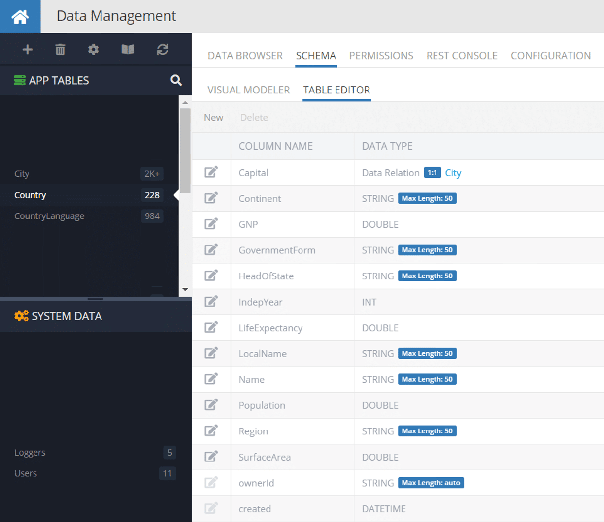
You can see the Country table in our Table Editor (previously our Schema Editor) below, with the Capital relation column at the top.

City

In the City table, the Country column will be a 1:1 relation with the country to which the city belongs. If you wanted to get more accurate, you could make this a 1:N (one-to-many) relation for any cities that are contested by multiple nations or overlap national borders.

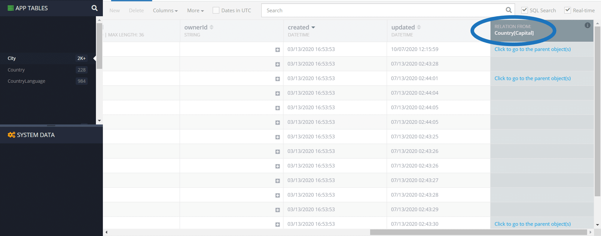
Below, we can see how the Capital relation appears within the City table:

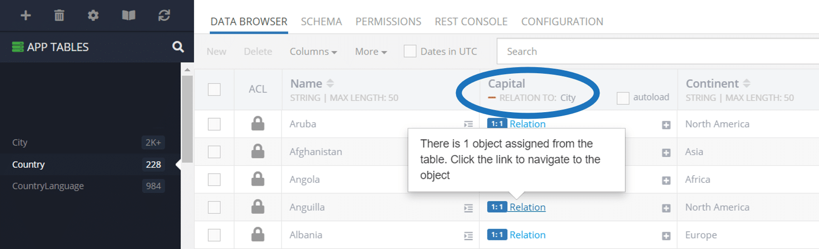
…and how the Capital column appears in the Country table:

CountryLanguage

Finally, in the CountryLanguage table, we have a couple options we could choose. We could create an 1:N relation, where each language can be connected to multiple countries.

Our second option is to create multiple instances of languages, allowing only a 1:1 relation between the language and the country while having a 1:N relationship between country and language. This is the approach we will take in this article.

Once we have these tables built, we can look at our schema visually to review the relationships:

Summary

The new Visual Data Modeler provides you with a much easier means of reviewing the relationships between tables in your database. This feature is live now and comes standard with all Backendless products.

Our goal is to make the complex simple. We hope this new feature will make working with data relations easier than ever.

Thanks for reading, and Happy Codeless Coding!